Theory

The RT1 module provides a method for calculating the scattered radiation from a uniformly illuminated rough surface covered by a homogeneous layer of tenuous media. The following sections are intended to give a general overview of the underlying theory of the RT1 module. A more general discussion on the derivation of the used results can be found in [QuWa16]. Details on how to define the scattering properties of the covering layer and the ground surface within the RT1-module are given in Model Specification.

The utilized theoretical framework is based on applying the Radiative Transfer Equation (RTE) (1) to the geometry shown in Fig. 1.

(1)\[\cos(\theta) \frac{\partial I_f(r,\theta,\phi)}{\partial r} = -\kappa_{ex} I_f(r,\theta,\phi) + \kappa_s \int\limits_{0}^{2\pi}\int\limits_{0}^{\pi/2} I_f(r,\theta',\phi') \hat{p}(\theta,\phi,\theta',\phi') \sin(\theta') d\theta' d\phi'\]

The individual variables are hereby defined as follows:

• \(\theta\) denotes the polar angle in a spherical coordinate system

• \(\phi\) denotes the azimuth angle in a spherical coordinate system

• \(r\) denotes the distance within the covering layer

• \(I_f(r,\theta,\phi)\) denotes the specific intensity at a distance \(r\) within the covering layer propagating in direction \((\theta,\phi)\).

• \(\kappa_{ex}\) denotes the extinction-coefficient (i.e. extinction cross section per unit volume)

• \(\hat{p}(\theta,\phi,\theta',\phi')\) denotes the scattering phase-function of the constituents of the covering layer

Note

To remain consistent with [QuWa16], the arguments of the functions \(\hat{p}(\theta,\phi,\theta',\phi')\) and \(BRDF(\theta,\phi,\theta',\phi')\) are defined as angles with respect to a spherical coordinate system in the following discussion. Within the RT1-module however, the functions are defined with respect to the associated zenith-angles!

A relationship between the module-functions and the functions within the subsequent discussion is therefore given by:

SRF.brdf(t_0,t_ex,p_0,p_ex) \(\hat{=} ~BRDF(\pi - \theta_0, \phi_0, \theta_{ex},\phi_{ex}) \quad\) and \(\mbox{}\quad\) V.p(t_0,t_ex,p_0,p_ex) \(\hat{=} ~\hat{p}(\pi - \theta_0, \phi_0, \theta_{ex},\phi_{ex})\)

Problem Geometry and Boundary Conditions

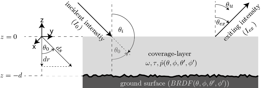
Fig. 1 Illustration of the chosen geometry within the RT1-module (adapted from [QuWa16])

As shown in Fig. 1, the considered problem geometry is defined as a rough surface covered by a homogeneous layer of a scattering and absorbing medium.

In order to be able to solve the RTE (1), the boundary-conditions are specified as follows:

• The top of the covering layer is uniformly illuminated at a single incidence-direction:

(2)\[I_0(z=0,\theta,\phi) = \frac{I_0}{\sin(\theta)} \delta(\theta - \theta_i) \delta(\phi - \phi_i)\]

• Radiation impinging at the ground surface is reflected upwards according to its associated Bidirectional Reflectance Distribution Function (BRDF)

(3)\[I^+(z=-d, \theta, \phi) = \int_{0}^{2\pi} \int_{0}^{\pi} I^-(z=-d, \theta, \phi) BRDF(\theta,\phi,\theta',\phi') \sin(\theta') d\theta' d\phi'\]

The superscripts \(I^\pm\) hereby indicate a separation between upwelling \((+)\) and downwelling \((-)\) intensity.

The additional specifications of the covering layer and the ground surface are summarized as follows:

Parameters used to describe the scattering properties of the covering layer

Scattering Phase Function: (i.e. normalized differential scattering cross section)

(4)\[\hat{p}(\theta,\phi,\theta',\phi') \qquad \textrm{with} \qquad \int\limits_0^{2\pi} ~ \int\limits_{0}^{\pi} \hat{p}(\theta,\phi,\theta',\phi') \sin(\theta') d\theta' d\phi' = 1\]

Optical Depth:

(5)\[\tau = \kappa_{ex} ~ d = (\kappa_{s} + \kappa_{a}) ~ d\]

where \(\kappa_{ex}\) is the extinction coefficient (i.e. extinction cross section per unit volume) , \(\kappa_{s}\) is the scattering coefficient (i.e. scattering cross section per unit volume) , \(\kappa_{a}\) is the absorption coefficient (i.e. absorption cross section per unit volume) and \(d\) is the total height of the covering layer.

Single Scattering Albedo:

(6)\[\omega = \frac{\kappa_{s}}{\kappa_{ex}} = \frac{\kappa_{s}}{\kappa_{s} + \kappa_{a}} \leq 1\]

Parameters used to describe the scattering properties of the ground surface

Bidirectional Reflectance Distribution Function:

(7)\[BRDF(\theta,\phi,\theta',\phi') \qquad \textrm{with} \qquad \int\limits_0^{2\pi} ~ \int\limits_{0}^{\pi/2} BRDF(\theta,\phi,\theta',\phi') \cos(\theta') \sin(\theta') d\theta' d\phi' = R(\theta,\phi) \leq 1\]

where \(R(\theta,\phi)\) denotes the Directional-Hemispherical Reflectance of the ground surface.

TBD: perhaps describe also normalization conditions for p and BRDF

First-order solution to the RTE

Incorporating the above specifications, a solution to the RTE is obtained by assuming that the scattering coefficient \(\kappa_s\) of the covering layer is small (i.e. \(\kappa_s\ll 1\)). Using this assumption, the RTE is expanded into a series with respect to powers of \(\kappa_s\), given by:

(8)\[I^+ = I_{\textrm{surface}} + I_{\textrm{volume}} + I_{\textrm{interaction}} + (I_{svs}) + \mathcal{O}(\kappa_s^2)\]

where the individual terms (representing the contributions to the scattered intensity at the top of the covering layer) can be interpreted as follows:

• \(I_{\textrm{surface}}\): radiation scattered once by the ground surface

• \(I_{\textrm{volume}}\): radiation scattered once within the covering layer

• \(I_{\textrm{interaction}}\): radiation scattered once by the ground surface and once within the covering layer

• \(I_{svs}\): radiation scattered twice by the ground surface and once within the covering layer

  (This contribution is assumed to be negligible due to the occurrence of second order surface-scattering)

After some algebraic manipulations the individual contributions are found to be given by (details can be found in [QuWa16]):

(9)\[I_{\textrm{surface}}(\theta_0, \phi_0, \theta_{ex}, \phi_{ex}) = I_0 e^{-\frac{\tau}{\cos(\theta_0)}} ~ e^{-\frac{\tau}{\cos(\theta_{ex})}} \cos(\theta_0) BRDF(\pi-\theta_0, \phi_0, \theta_{ex}, \phi_{ex})\]

(10)\[I_{\textrm{volume}}(\theta_0, \phi_0, \theta_{ex}, \phi_{ex}) = I_0 ~\omega ~ \frac{\cos(\theta_0)}{\cos(\theta_0) + \cos(\theta_{ex})} \left( 1 - e^{-\frac{\tau}{\cos(\theta_0)}} ~ e^{-\frac{\tau}{\cos(\theta_{ex})}} \right) \hat{p}(\pi-\theta_0, \phi_0, \theta_{ex}, \phi_{ex})\]

(11)\[I_{\textrm{interaction}}(\theta_0, \phi_0, \theta_{ex}, \phi_{ex}) = I_0 ~ \cos(\theta_0) ~ \omega \left\lbrace e^{-\frac{\tau}{\cos(\theta_{ex})}} F_{int}(\theta_0,\theta_{ex}) + e^{-\frac{\tau}{\cos(\theta_{ex})}} F_{int}(\theta_{ex},\theta_{0}) \right\rbrace\]

(12)\[\textrm{with} \qquad \qquad F_{int}(\theta_0, \phi_0, \theta_{ex}, \phi_{ex}) = \int\limits_0^{2\pi} \int\limits_0^\pi \frac{\cos(\theta)}{\cos(\theta_0)-\cos(\theta)} \left( e^{-\frac{\tau}{\cos(\theta_0)}} - e^{-\frac{\tau}{\cos(\theta)}} \right) ~ \hat{p}(\theta_0, \phi_0, \theta , \phi) BRDF(\pi - \theta, \phi, \theta_{ex}, \phi_{ex}) \sin(\theta) d\theta d\phi\]

Evaluation of the interaction-contribution

In order to analytically evaluate the remaining integral appearing in the interaction-term, the BRDF and the scattering phase-function of the covering layer are approximated via a Legendre-series in a (possibly generalized) scattering angle of the form:

(13)\[BRDF(\theta, \phi, \theta_{s}, \phi_{s}) = \sum_{n=0}^{N_b} b_n P_n(\cos(\Theta_{a_b}))\]

(14)\[\hat{p}(\theta, \phi, \theta_{s}, \phi_{s}) = \sum_{n=0}^{N_p} p_n P_n(\cos(\Theta_{a_p}))\]

where \(P_n(x)\) denotes the \(\textrm{n}^\textrm{th}\) Legendre-polynomial and the generalized scattering angle \(\Theta_a\) is defined via:

(15)\[\cos(\Theta_a) = a_0 \cos(\theta) \cos(\theta_{s}) + \sin(\theta) \sin(\theta_{s}) \left[a_1 \cos(\phi) \cos(\phi_{s}) + a_2 \sin(\phi) \sin(\phi_{s}) \right]\]

where \(\theta ,\phi\) are the polar- and azimuth-angles of the incident radiation, \(\theta_{s}, \phi_{s}\) are the polar- and azimuth-angles of the scattered radiation and \(a_1,a_2\) and \(a_3\) are constants that allow consideration of off-specular and anisotropic effects within the approximations.

Once the \(b_n\) and \(p_n\) coefficients are known, the method developed in [QuWa16] is used to analytically solve \(I_{\textrm{interaction}}\).

This is done in two steps:

First, the so-called fn-coefficients are evaluated which are defined via:

(16)\[\int_{0}^{2\pi} \hat{p}(\theta_0,\phi_0,\theta,\phi)BRDF(\pi - \theta, \phi, \theta_{ex},\phi_{ex}) d\phi = \sum_{n=0}^{N_b + N_p} f_n(\theta_0,\phi_0,\theta_{ex},\phi_{ex}) \cos(\theta)^n\]

Second, \(I_{\textrm{interaction}}\) is evaluated using the analytic solution to the remaining \(\theta\)-integral for a given set of fn-coefficients as presented in [QuWa16].

Example

In the following, a simple example on how to evaluate the fn-coefficients is given. The ground is hereby defined as a Lambertian-surface and the covering layer is assumed to consist of Rayleigh-particles. Thus, we have: (\(R_0\) hereby denotes the diffuse albedo of the surface)

• \(BRDF(\theta, \phi, \theta_{ex},\phi_{ex}) = \frac{R_0}{\pi}\)

• \(p(\theta, \phi, \theta_{ex},\phi_{ex}) = \frac{3}{16\pi} (1+\cos(\Theta)^2) \quad\) with \(\mbox{}\quad\) \(\cos(\Theta) = \cos(\theta)\cos(\theta_{ex}) + \sin(\theta)\sin(\theta_{ex})\cos(\phi - \phi_{ex})\)

(17)\[\begin{split}INT &= \int_0^{2\pi} p(\theta_0, \phi_0, \theta,\phi) * BRDF(\pi-\theta, \phi, \theta_{ex},\phi_{ex}) d\phi \\ &= \frac{3 R_0}{16 \pi^2} \int\limits_{0}^{2\pi} (1+[\cos(\theta_0)\cos(\theta) + \sin(\theta_0)\sin(\theta)\cos(\phi_0 - \phi)]^2) d\phi \\ &= \frac{3 R_0}{16 \pi^2} \int\limits_0^{2\pi} (1+ \mu_0^2 \mu^2 + 2 \mu_0 \mu \sin(\theta_0) \sin(\theta) \cos(\phi_0 - \phi) + (1-\mu_0)^2(1-\mu)^2 \cos(\phi_0 - \phi)^2 d\phi\end{split}\]

where the shorthand-notation \(\mu_x = \cos(\theta_x)\) has been introduced.

The above integral can now easily be solved by noticing:

(18)\[\begin{split}\int\limits_0^{2\pi} \cos(\phi_0 - \phi)^n d\phi = \left\lbrace \begin{matrix} 2 \pi & \textrm{for } n=0 \\ 0 & \textrm{for } n=1 \\ \pi & \textrm{for } n=2 \end{matrix} \right.\end{split}\]

Using some algebraic manipulations we therefore find:

(19)\[\begin{split}INT = \frac{3 R_0}{16\pi} \Big[ (3-\mu_0^2) + (3 \mu_0 -1) \mu^2 \Big] = \sum_{n=0}^2 f_n ~ \mu^n \\ \\ \Rightarrow \quad f_0 = \frac{3 R_0}{16\pi}(3-\mu_0^2) \qquad f_1 = 0 \qquad f_2 = \frac{3 R_0}{16\pi}(3 \mu_0 -1) \qquad f_n = 0 ~ \forall ~n>2\end{split}\]

An IPython-notebook that uses the RT1-module to evaluate the above fn-coefficients can be found HERE

References

QuWa16(1,2,3,4,5,6)

R.Quast and W.Wagner, “Analytical solution for first-order scattering in bistatic radiative transfer interaction problems of layered media,” Appl.Opt.55, 5379-5386 (2016)