Model Specification
Evaluation Geometries
From the general definition of the fn-coefficients (16) it is apparent that they are in principle dependent on \(\theta_0,\phi_0,\theta_{ex}\) and \(\phi_{ex}\). If the series-expansions ((13) and (14)) contain a high number of Legendre-polynomials, the resulting fn-coefficients turn out to be rather lengthy and moreover their evaluation might consume a lot of time. Since usually one is only interested in an evaluation with respect to a specific (a-priori known) geometry of the measurement-setup, the rt1-module incorporates a parameter that allows specifying the geometry at which the results are being evaluated. This generally results in a considerable speedup for the fn-coefficient generation.
The measurement-geometry is defined by the value of the geometry-parameter of the RT1-class object:
R = RT1(... , geometry = '????')
The geometry-parameter must be a 4-character string that can take one of the following possibilities:
'mono'for Monostatic Evaluationany combination of
'f'and'v'for Bistatic Evaluation
To clarify the definitions, the used angles are illustrated in Fig. 2.
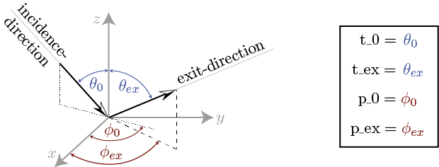
Fig. 2 Illustration of the used incidence- and exit-angles
Monostatic Evaluation
Monostatic evaluation refers to measurements where both the transmitter and the receiver are at the same location.
In terms of spherical-coordinate description, this is equal to (see Fig. 2):
Since a monostatic setup drastically simplifies the evaluation of the fn-coefficients, setting the module exclusively to monostatic evaluation results in a considerable speedup.
The module is set to be evaluated at monostatic geometry by setting:
R = RT1(... , geometry = 'mono')
Note
If
geometryis set to'mono', the values oft_exandp_exhave no effect on the calculated results since they are automatically set tot_ex = t_0andp_ex = p_0 + PiFor azimuthally symmetric phase-functions 1, the value of
p_0has no effect on the calculated result and the best performance will be achieved by settingp_0 = 0.
- 1
This referrs to any phase-function whose generalized scattering angle parameters satisfy
a[0] = ?, a[1] == a[2] = ?. The reason for this simplification stems from the fact that the azimuthal dependency of a generalized scattering angle witha[1] == a[2]can be expressed in terms of \(\cos(\phi_0 - \phi_{ex})^n\). For the monostatic geometry this reduces to \(\cos(\pi)^n = 1\) independent of the choice of \(\phi_0\).
Bistatic Evaluation
Any possible bistatic measurement geometry can be chosen by manually selecting the angles that shall be treated symbolically (i.e. variable), and those that are treated as numerical constants (i.e. fixed).
The individual characters of the geometry-string hereby represent
the properties of the incidence- and exit angles (see Fig. 2) in the order of appearance within the RT1-class element, i.e.:
geometry[0] ... t_0
geometry[1] ... t_ex
geometry[2] ... p_0
geometry[3] ... p_ex
- The character
'f'indicates a fixed angle The given numerical value of the angle will be used rather than it’s symbolic representation to speed up evaluation.
The resulting fn-coefficients are only valid for the chosen specific value of the angle.
- The character
- The character
'v'indicates a variable angle The angle will be treated symbolically when evaluating the fn-coefficients in order to provide an analytic representation of the interaction-term where the considered angle is treated as a variable.
The resulting fn-coefficients can be used for any value of the angle.
- The character
As an example, the choice geometry = 'fvfv' represents a measurement setup where the surface is illuminated at
constant (polar- and azimuth) incidence-angles and the location of the receiver is variable both in azimuth- and polar direction.
Note
Whenever a single angle is set fixed, the calculated fn-coefficients are only valid for this specific choice!
If the chosen scattering-distributions reqire an approximation with a high degree of Legendre-polynomials, evaluating the interaction-contribution with
geometry = 'vvvv'might take considerable time since the resulting fn-coefficients are very long symbolic expressions.
Linear combination of scattering distributions
Aside of directly specifying the scattering distributions by choosing one of the implemented functions, the RT1-module has a method to define linear-combinations of scattering distributions to allow consideration of more complex scattering characteristics.
An IPython-notebook that shows the basic usage of linear-combinations within the RT1-module is provided HERE .
Combination of volume-scattering phase-functions
Linear-combination of volume-scattering phase-functions is used to generate a combined volume-class element of the form:
where \(\hat{p}_n(\cos(\Theta_{a_n}))\) denotes the scattering phase-functions to be combined, \(\cos(\Theta_{a_n})\) denotes the individual scattering angles (15) used to define the scattering phase-functions \(w_n\) denotes the associated weighting-factors, \(p_k^{(n)}\) denotes the \(\textrm{k}^{\textrm{th}}\) Legendre-expansion-coefficient (14) of the \(\textrm{n}^{\textrm{th}}\) phase-function and \(\hat{P}_k(x)\) denotes the \(\textrm{k}^{\textrm{th}}\) Legendre-polynomial.
Note
Since a volume-scattering phase-function must obey the normalization condition:
and each individual phase-function that is combined already satisfies this condition, the weighting-factors \(w_n\) must equate to 1, i.e.:
Within the RT1-module, linear-combination of volume-scattering phase-functions is performed by the LinCombV(omega, tau, Vchoices) function:
from rt1.volume import LinCombV
In order to generate a combined phase-function, one must provide the optical depth tau, the single-scattering albedo omega
and a list of volume-class elements along with a set of weighting-factors (Vchoices) of the form:
Vchoices = [ [weighting-factor , function] , [weighting-factor , function] , ... ]
Once the functions and weighting-factors have been defined, the combined phase-function is generated via:
V = LinCombV(tau, omega, Vchoices)
The resulting volume-class element can now be used completely similar to the pre-defined scattering phase-functions.
Note
Since one can combine functions with different choices for the generalized scattering angle (i.e. the a-parameter),
and different numbers of expansion-coefficients (the ncoefs-parameter) LinCombV() will automatically combine
the associated Legendre-expansions based on the choices for a and ncoefs.
The parameters V.a, V.scat_angle() and V.ncoefs of the resulting volume-class element are therefore NOT representative for the generated combined phase-function!
Combination of BRDF’s
Linear-combination of BRDF’s is used to generate a combined surface-class element of the form:
where \(BRDF_n(\cos(\Theta_{a_n}))\) denotes the BRDF’s to be combined, \(\cos(\Theta_{a_n})\) denotes the individual scattering angles (15) used to define the BRDF’s \(w_n\) denotes the associated weighting-factors, \(b_k^{(n)}\) denotes the \(\textrm{k}^{\textrm{th}}\) Legendre-expansion-coefficient (13) of the \(\textrm{n}^{\textrm{th}}\) BRDF and \(\hat{P}_k(x)\) denotes the \(\textrm{k}^{\textrm{th}}\) Legendre-polynomial.
Note
Since a BRDF must obey the following normalization condition:
there is in principle no restriction on the weighting-factors for combination of BRDF’s!
It is however important to notice that the associated hemispherical reflectance \(R(\theta_0,\phi_0)\) must always be lower or equal to 1.
In order to provide a simple tool that allows validating the above condition, the function RT1.Plots().hemreflect() numerically evaluates
the hemispherical reflectance using a simple Simpson-rule integration-scheme and generates a plot that displays \(R(\theta_0,\phi_0)\).
Within the RT1-module, linear-combination of BRDF’s is performed by the LinCombSRF(omega, tau, SRFchoices) function:
from rt1.surface import LinCombSRF
In order to generate a combined phase-function, one must provide a list of surface-class elements along with a set of weighting-factors (SRFchoices) of the form:
SRFchoices = [ [weighting-factor , function] , [weighting-factor , function] , ... ]
Once the functions and weighting-factors have been defined, the combined BRDF is generated via:
SRF = LinCombSRF(SRFchoices)
The resulting surface-class element can now be used completely similar to the pre-defined BRDF’s.
Note
Since one can combine functions with different choices for the generalized scattering angle (i.e. the a-parameter),
and different numbers of expansion-coefficients (the ncoefs-parameter) LinCombSRF() will automatically combine
the associated Legendre-expansions based on the choices for a and ncoefs.
The parameters SRF.a, SRF.scat_angle() and SRF.ncoefs of the resulting surface-class element are therefore NOT representative for the generated combined BRDF!
Current limitations
The list of pre-defined BRDF’s and volume-scattering phase-functions currently contains only few example of possible choices and is intended to be extended. For example the possibility of using delta-peaked scattering-distributions is contemplated for future versions of the code.
If the expansion-coefficients of the BRDF and volume-scattering phase-function exceed a certain number (approx. ncoefs > 20) one might run into numerical precision errors.